People come in a variety of shapes and sizes. Get a few million people together in one place, say in Rhode Island or South Carolina, and it would be impossible to predict what a single person selected from either state would be like. Try to compare all Rhode Islanders to all South Carolinians and the task gets even more complex. Obviously, something is needed to simplify the process, and that’s why we have statistics.

The first step is to decide on a measurement, such as weight. Yes, this ignores that Mary Jane in SC has freckles and John in RI has a tattoo but we have to focus on something or we can’t make a comparison. Unfortunately, even after focusing on a single measurement, we still have two different populations of data points consisting of millions of wildly different numbers. These populations include everything from two pound preemies to 400+ pound bubbas.

Again, we must simplify and so we’ll focus on a parameter that can characterize the weights of all individuals in a population. A parameter is a number which summarizes a specific characteristic generated from measurements of every member of a population. Using a parameter it’s possible to represent a property of an entire population with a single number instead of millions of individual data points.

There are a number of possible parameters to choose from such as the median, mode, or interquartile range. Each is calculated in a different manner and illuminates the data from a different point of view. We’ll use the mean, because it’s one of the most useful and widely used. In spite of its harsh sounding name it has a very nice effect on helping us understand populations.

The mean, or average, summarizes something called central tendency. This is a fancy way of saying what’s typical, normal, or expected in a population. If all the data points were plotted on a line segment the most typical values would be found somewhere near the center of the line segment, hence, the term central tendency.

Of course central tendency isn’t the only issue. There’s also the issue of variability or spread. We like to call this wildness although, admittedly, wildness is not a standard term. However, wildness seems appropriate, since, individuals drawn from populations with lots of variability or spread tend to be wildly unpredictable.

While the mean gives us a single number to describe a complex population, it’s, unfortunately, a parameter. We have to use every single data point in a population to calculate a parameter. With millions of data points to collect, this could be a real problem. By the time we got all the measurements, the two pound preemies might have turned into 400+ pound adults.

The solution is to use a randomly chosen sample of the population and calculate a statistic. Statistics are always based on samples. We would carefully collect a few data points chosen at random and calculate a sample mean. We’ll call this statistic x-bar. Clearly, x-bar is not a parameter since it’s not calculated from the entire population. It’s only an estimate of the parameter.

Fig. 1) Histogram of Population - Uniform Distribution: population = 10,000; mean = 5.013; std dev 2.897   Fig. 2) Sampling Distribution n = 2: number of samples = 2010; mean = 4.995; std dev 2.011; std error = 2.048   Fig. 3) Sampling Distribution n = 10: number of samples = 2010; mean = 5.018; std dev 0.906; std error = 0.917   Fig. 4) Sampling Distribution n = 50: number of samples = 2010; mean = 4.999; std dev 0.411; std error = 0.410

If we selected another sample and calculated a second x-bar we might find that it differs considerably from the first. By their nature, random samples can sometimes give unexpected results even when flawlessly collected. For example, the first could be made up mostly of preemies while the second could be made up of sumo wrestlers. While such extremes are unlikely, selecting large sized samples would prevent them. After all, there are just so many preemies and sumo wrestlers available. A large sized sample could never be made up entirely of either preemies or sumo wrestlers.

Ultimately, if one sample mean or x-bar is wildly different from another we would not be any better off than trying to look at the entire population. Obviously, we need to understand just how wild or variable sample means or x-bars are likely to be.

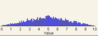
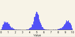
To understand the wildness of samples, we would choose thousands of samples, calculate an x-bar for each, and display the x-bars in a histogram. We call this histogram a sampling distribution and when we look at it we see something which is truly amazing. Sampling distributions tend to be far less variable or wild than the populations they are drawn from (See Fig.s 1, 2, 3 and 4.) They also have essentially the same mean as the population.

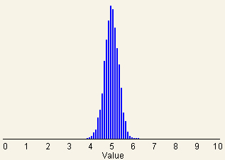
What’s more, sampling distributions drawn from a uniformly distributed population start to look like normal distributions even with a sample size as small as 2 (see Fig. 2). If the sample size is large enough they form nearly perfect normal distributions. This may not seem Earth shattering but it’s really quite profound. Anytime we know data follows a normal distribution, we immediately have a lot more confidence that we can predict how the data will behave.

The situation is similar to hiring Mary Jane, who has a master’s degree in computer science versus Jim Bob who says he can compute. Jim Bob may turn out to be better at creating software. However, by knowing that Mary Jane has a master’s degree we feel a lot more confident in our ability to predict her programming capability.

Although the figures at right are for a population with a uniform distribution, the central limit theorem works well regardless of the population's distribution. The applet illustrates this nicely. It includes a highly skewed as well as a bimodal population. With a large sample size of 100, the histogram of the sampling distribution in the applet looks spike-like. However, normal distributions look this way when they have a  small standard deviations.

It would be highly annoying if we had to generate an entire sampling distribution every time we want to be sure that our statistic based on a sample really is less wild than the data points in the population. Fortunately, we know this ahead of time, thanks to the (arguably) second most profound principle in all of statistics, the central limit theorem (the law of large numbers being the first).

The central limit theorem tells us that a sampling distribution always has significantly less wildness than the population it’s drawn from. Additionally, the sampling distribution will act more and more like normal distribution as the sample size is increased, even when the population itself is not normally distributed!

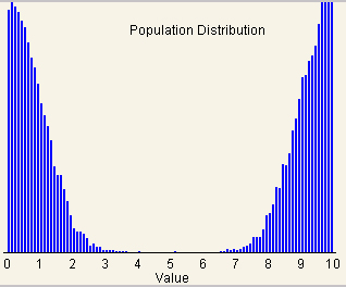
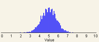
If we use standard deviation as a measurement of wildness the standard deviation of a sampling distribution (sometimes called the standard error) is as follows:

For example, the sampling distribution for a sample size of 100 will have 1/10 as much wildness or variability as the population. In other words, an x-bar based on a relatively small sample of 100 will do a surprisingly consistent job of estimating the true mean. Again, it’s not particularly important for the population to be normally distributed.

When we look at equation (1) we notice something very profound because it’s missing. There’s no term for the size of the population. This means that the reduction in wildness depends only on the sample size. In other words, a statistic based on a sample size of say 2000 will be just as meaningful if it’s drawn from a population of 20,000,000,000 as it will be if it’s drawn from a population of 20,000. Population size does not matter as long as it’s at least 10 times larger than the sample.

If the central limit theorem didn’t exist, it would not be possible to use statistics. We would be unable to reliably estimate a parameter like the mean by using an average derived from a much smaller sample. This would all but shut down research in the social sciences and the evaluation of new drugs since these depend on statistics. It would invalidate the use of polls and completely alter the nature of marketing research not to mention politics.

Thanks to the central limit theorem, we can be sure that a mean or x-bar based on a reasonably large randomly chosen sample will be remarkably close to the true mean of the population. If we need more certainty we need only increase the sample size. What’s more, it does not matter if we are characterizing a city, state, or the entire United States, we can use the same sample size. It will give the same level of certainty regardless of the population size.

For further Information

Sampling Distribution Applet: This applet can also be very helpful for understanding sampling distributions. However, be aware that in it the sampling distribution's vertical scale changes with the number of samples and the sample size only goes up to 25. This hides the dramatic narrowing effect on the sampling distribution caused by increasing sample size. The above applet plots population and sampling distributions on exactly the same scales and allows sample sizes of 100, all of  which make the narrowing effect highly visible. Both applets are correct although they look different due to differences in scales.

< Return to Contents