|
|
Type I and Type II Errors -
Making Mistakes in the Justice System |
|
|
Ever wonder how someone in America can be arrested if they really are
presumed innocent, why a defendant is found not guilty instead of
innocent, or why Americans put up with a justice system which sometimes
allows criminals to go free on technicalities? These questions can be
understood by examining the similarity of the American justice system to
hypothesis testing in statistics and the two types of errors it can
produce. (This discussion assumes that the reader has at least been
introduced to the normal distribution and its use in hypothesis testing.
Also please note that the American justice system is used for convenience.
Others are similar in nature such as the British system which inspired the
American system)
True, the trial process does not use numerical values
while hypothesis testing in statistics does, but both share at least four
common elements (other than a lot of jargon that sounds like double talk):
- The alternative hypothesis - This is the
reason a criminal is arrested. Obviously the police don't think the
arrested person is innocent or they wouldn't arrest him. In statistics
the alternative hypothesis is the hypothesis the researchers wish to
evaluate.
- The null hypothesis - In the criminal justice
system this is the presumption of innocence. In both the judicial system
and statistics the null hypothesis indicates that the suspect or
treatment didn't do anything. In other words, nothing out of the
ordinary happened The null is the logical opposite of the alternative. For example "not white" is the logical opposite of white.
Colors such as red, blue and green as well as black all qualify as "not
white".
- A standard of judgment - In the justice system
and statistics there is no possibility of absolute proof and so a
standard has to be set for rejecting the null hypothesis. In the justice
system the standard is "a reasonable doubt". The null hypothesis has to
be rejected beyond a reasonable doubt. In statistics the standard is the
maximum acceptable probability that the effect is due to random
variability in the data rather than the potential cause being
investigated. This standard is often set at 5% which is called the alpha
level.
- A data sample - This is the information
evaluated in order to reach a conclusion. As mentioned earlier, the data
is usually in numerical form for statistical analysis while it may be in
a wide diversity of forms--eye-witness, fiber analysis, fingerprints,
DNA analysis, etc.--for the justice system. However in both cases there
are standards for how the data must be collected and for what is
admissible. Both statistical analysis and the justice system operate on
samples of data or in other words partial information because, let's
face it, getting the whole truth and nothing but the truth is not
possible in the real world.
It only takes one good piece of evidence to send a
hypothesis down in flames but an endless amount to prove it correct. If
the null is rejected then logically the alternative hypothesis is
accepted. This is why both the justice system and statistics concentrate
on disproving or rejecting the null hypothesis rather than proving the
alternative. It's much easier to do. If a jury
rejects the presumption of innocence, the defendant is pronounced guilty.
Type I errors: Unfortunately, neither the legal
system or statistical testing are perfect. A jury sometimes makes an error
and an innocent person goes to jail. Statisticians, being highly
imaginative, call this a type I error. Civilians call it a travesty.
In the justice system, failure to reject the presumption
of innocence gives the defendant a not guilty verdict. This means only
that the standard for rejecting innocence was not met. It does not mean
the person really is innocent. It would take an endless amount of evidence
to actually prove the null hypothesis of innocence.
Type II errors: Sometimes, guilty people are set
free. Statisticians have given this error the highly imaginative name,
type II error.
Americans find type II errors disturbing but not as
horrifying as type I errors. A type I error means that not only has an
innocent person been sent to jail but the truly guilty person has gone
free. In a sense, a type I error in a trial is twice as bad as a type II
error. Needless to say, the American justice system puts a lot of emphasis
on avoiding type I errors. This emphasis on avoiding type I errors,
however, is not true in all cases where statistical hypothesis testing is
done.
In statistical hypothesis testing used for quality
control in manufacturing, the type II error is considered worse than a
type I. Here the null hypothesis indicates that the product satisfies the
customer's specifications. If the null hypothesis is rejected for a batch
of product, it cannot be sold to the customer. Rejecting a good batch by
mistake--a type I error--is a very expensive error but not as expensive as
failing to reject a bad batch of product--a type II error--and shipping it
to a customer. This can result in losing the customer and tarnishing the
company's reputation.
|
Justice System - Trial |
|
Defendant Innocent |
Defendant Guilty |
|
Reject Presumption
of Innocence (Guilty Verdict) |
Type I Error |
Correct |
|
Fail to Reject
Presumption of Innocence (Not Guilty Verdict) |
Correct |
Type II
Error |
|
|
|
Statistics - Hypothesis Test |
|
Null Hypothesis True |
Null Hypothesis False |
|
Reject Null
Hypothesis |
Type I Error |
Correct |
|
Fail to Reject Null
Hypothesis |
Correct |
Type II
Error |
|
|
|
In the criminal justice system a
measurement of guilt or innocence is packaged in the form of a witness,
similar to a data point in statistical analysis. Using this comparison we
can talk about sample size in both trials and hypothesis tests. In a
hypothesis test a single data point would be a sample size of one and ten
data points a sample size of ten. Likewise, in the justice system one
witness would be a sample size of one, ten witnesses a sample size ten,
and so forth.
Impact on a jury is going to depend on the
credibility of the witness as well as the actual testimony. An articulate
pillar of the community is going to be more credible to a jury than a
stuttering wino, regardless of what he or she says.
The normal distribution shown in figure 1
represents the distribution of testimony for all possible witnesses in a
trial for a person who is innocent. Witnesses represented by the left hand
tail would be highly credible people who are convinced that the person is
innocent. Those represented by the right tail would be highly credible
people wrongfully convinced that the person is guilty.
At first glace, the idea that highly
credible people could not just be wrong but also adamant about their
testimony might seem absurd, but it happens. According to the
innocence
project, "eyewitness misidentifications contributed to over 75% of the
more than 220 wrongful convictions in the United States overturned by
post-conviction DNA evidence." Who could possibly be more credible than a
rape victim convinced of the identity of her attacker, yet even here
mistakes have been documented.
For example, a rape victim mistakenly
identified
John Jerome White as her attacker even though the actual perpetrator
was in the lineup at the time of identification. Thanks to DNA evidence
White was eventually exonerated, but only after wrongfully serving 22
years in prison.
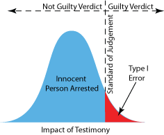
If the standard of judgment for evaluating
testimony were positioned as shown in figure 2 and only one witness
testified, the accused innocent person would be judged guilty (a type I
error) if the witnesses testimony was in the red area. Since the normal
distribution extends to infinity, type I errors would never be zero even
if the standard of judgment were moved to the far right. The only way to
prevent all type I errors would be to arrest no one. Unfortunately this
would drive the number of unpunished criminals or type II errors through
the roof.
|
|
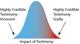 |
figure 1. Distribution of possible witnesses in
a trial when the accused is innocent
|
|
|
|
figure 2. Distribution of possible witnesses in
a trial when the accused is innocent, showing the probable outcomes
with a single witness.
|
|
|
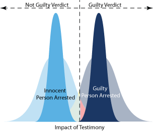
Figure 3 shows what happens not only to innocent
suspects but also guilty ones when they are arrested and tried for crimes.
In this case, the criminals are clearly guilty and face certain punishment
if arrested.
|
 |
|
 |
| figure 3. Distribution of
possible witnesses in a trial showing the probable outcomes with a
single witness if the accused is innocent or obviously guilty.. |
|
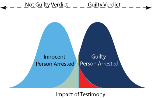
figure 4. Distribution of possible
witnesses in a trial showing the probable outcomes with a single
witness if the accused is innocent or not clearly guilty.. |
| |
|
|
|
If the police bungle the investigation and
arrest an innocent suspect, there is still a chance that the
innocent person could go to jail. Also, since the normal
distribution extends to infinity in both positive and negative
directions there is a very slight chance that a guilty person
could be found on the left side of the standard of judgment and
be incorrectly set free.
Unfortunately, justice is often not as
straightforward as illustrated in figure 3. Figure 4 shows the
more typical case in which the real criminals are not so clearly
guilty. Notice that the means of the two distributions are much
closer together. As before, if bungling police officers arrest
an innocent suspect there's a small chance that the wrong person
will be convicted. However, there is now also a significant
chance that a guilty person will be set free. This is
represented by the yellow/green area under the curve on the left
and is a type II error.
|
|
 |
| |
|
figure 5. The effects of increasing
sample size or in other words, number of independent witnesses. |
|
If the standard of judgment is moved to the
left by making it less strict the number of type II errors or
criminals going free will be reduced. This change in the
standard of judgment could be accomplished by throwing out the
reasonable doubt standard and instructing the jury to find the
defendant guilty if they simply think it's possible that she did
the crime. However, such a change would make the type I errors
unacceptably high. While fixing the justice system by moving the
standard of judgment has great appeal, in the end there's no
free lunch.
Fortunately, it's possible to reduce type I
and II errors without adjusting the standard of judgment. Juries
tend to average the testimony of witnesses. In other
words, a highly credible witness for the accused will counteract
a highly credible witness against the accused. So, although at
some point there is a diminishing return, increasing the number
of witnesses (assuming they are independent of each other) tends
to give a better picture of innocence or guilt.
Increasing sample size is an obvious way to
reduce both types of errors for either the justice system or a
hypothesis test. As shown in figure 5 an increase of sample size
narrows the distribution. Why? Because the distribution
represents the average of the entire sample instead of just a
single data point.
In hypothesis testing the sample size is
increased by collecting more data. In the justice system it's
increase by finding more witnesses. Obviously, there are
practical limitations to sample size. In the justice system
witnesses are also often not independent and may end up
influencing each other's testimony--a situation similar to
reducing sample size. Giving both the accused and the prosecution access to lawyers
helps make sure that no significant witness goes unheard, but
again, the system is not perfect.
About the only other way to decrease both the
type I and type II errors is to increase the reliability of the
data measurements or witnesses. For example the Innocence
Project has proposed
reforms on how lineups are performed. These include blind
administration, meaning that the police officer administering
the lineup does not know who the suspect is. That way the
officer cannot inadvertently give hints resulting in
misidentification.
The value
of unbiased, highly trained, top quality police investigators with
state of the art equipment should be obvious. There is no
possibility of having a type I error if the police never arrest
the wrong person. Of course, modern tools such as DNA testing are
very important, but so are properly designed and executed police
procedures and professionalism. The famous trial of O.
J. Simpson would have likely ended in a guilty verdict if the Los
Angeles Police officers investigating the crime had been beyond
reproach.
< Return to Contents
|
|
|
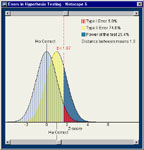
Statistical Errors
Applet
The applet below can alter both the
standard of judgment and distance between means for a
statistical hypothesis test. It calculates type I and type
II errors when you move the sliders. Like any analysis of
this type it assumes that the distribution for the null
hypothesis is the same shape as the distribution of the
alternative hypothesis.
Note, that the horizontal axis is set up
to indicate how many standard deviations a value is away
from the mean. Zero represents the mean for the
distribution of the null hypothesis.
When the sample size is one, the normal
distributions drawn in the applet represent the population
of all data points for the respective condition of Ho
correct or Ha correct. When the sample size is increased
above one the distributions become sampling distributions
which represent the means of all possible samples drawn
from the respective population. Standard error is simply
the standard deviation of a sampling distribution. Note
that this is the same for both sampling distributions
| Try
adjusting the sample size, standard of judgment (the
dashed red line), and position of the distribution for
the alternative hypothesis (Ha) and you will develop a
"feeling" for how they interact.
Note that a type I error is often
called alpha. The type II error is often called beta.
The power of the test = ( 100% - beta). |
|
 |
|
Applet 1. Statistical Errors |
|
Note: to run
the above applet you must have Java enabled in your
browser and have a Java runtime environment (JRE)
installed on you computer. If you have not installed a
JRE you can download it for free
here. |
|
|
|
|
|
|
|
|